HowTo

This section describes how to run each analysis function independently.

Calculate similarity

The example code:

"""
Created on Sat Apr  3 23:48:38 2021

@author: arsi
"""

import pandas as pd

from tscfat.Analysis.calculate_similarity import calculate_similarity

# load a dataframe and convert the index to datetime
df = pd.read_csv('/home/arsi/Documents/tscfat/Data/one_subject_data.csv',index_col=0)
df.index = pd.to_datetime(df.index)

# convert one column to a numpy array
name = 'positive'
ser = df[name].values.reshape(-1,1)

sim = calculate_similarity(ser)

The similarity matrix:

print(sim)
[[1.         0.8962963  0.8962963  ... 0.78317152 0.75467775 0.81208054]
 [0.8962963  1.         0.81208054 ... 0.86120996 0.82687927 0.8962963 ]
 [0.8962963  0.81208054 1.         ... 0.71810089 0.69407266 0.74233129]
 ...
 [0.78317152 0.86120996 0.71810089 ... 1.         0.95400788 0.95652174]
 [0.75467775 0.82687927 0.69407266 ... 0.95400788 1.         0.91435768]
 [0.81208054 0.8962963  0.74233129 ... 0.95652174 0.91435768 1.        ]]

Calculate Novelty

The example code:

"""
Created on Sat Apr  3 23:48:38 2021

@author: arsi
"""

import pandas as pd

from tscfat.Analysis.calculate_similarity import calculate_similarity
from tscfat.Analysis.calculate_novelty import compute_novelty

# load a dataframe and convert the index to datetime
df = pd.read_csv('/home/arsi/Documents/tscfat/Data/one_subject_data.csv',index_col=0)
df.index = pd.to_datetime(df.index)

# convert one column to a numpy array
name = 'positive'
ser = df[name].values.reshape(-1,1)

# similarity matrix
sim = calculate_similarity(ser)

# novelty score and kernel
nov, kernel = compute_novelty(sim,edge=7)

The novelty score:

print(nov)
[0.20766337 0.14769835 0.10181832 0.06656327 0.04818483 0.02417862
 0.01317275 0.01011372 0.00741401 0.00831496 0.00726132 ...
 ... 0.01400025 0.03109473 0.06095036 0.10315707 0.16478283 0.23854444]

Calculate Stability

The example code:

"""
Created on Sat Apr  3 23:48:38 2021

@author: arsi
"""

import pandas as pd

from tscfat.Analysis.calculate_similarity import calculate_similarity
from tscfat.Analysis.calculate_stability import compute_stability

# load a dataframe and convert the index to datetime
df = pd.read_csv('/home/arsi/Documents/tscfat/Data/one_subject_data.csv',index_col=0)
df.index = pd.to_datetime(df.index)

# convert one column to a numpy array
name = 'positive'
ser = df[name].values.reshape(-1,1)

# similarity matrix
sim = calculate_similarity(ser)

# stability score
stab = compute_stability(sim)

The stability score:

print(stab)
[0.         0.         0.         0.66850829 0.76100629 0.81208054
 0.84615385 0.8705036  0.88321168 0.88321168 0.8705036   ...
 ...        0.93316195 0.93556701 0.93556701 0.93556701 0.92602041
 0.90636704 0.87893462 0.8705036  0.84320557 0.         0.
 0.        ]

Plot Similarity

The example code:

"""
Created on Sat Apr  3 23:48:38 2021

@author: arsi
"""

import pandas as pd

from tscfat.Analysis.calculate_similarity import calculate_similarity
from tscfat.Analysis.calculate_novelty import compute_novelty
from tscfat.Analysis.calculate_stability import compute_stability
from tscfat.Analysis.plot_similarity import plot_similarity

# load a dataframe and convert the index to datetime
df = pd.read_csv('/home/arsi/Documents/tscfat/Data/one_subject_data.csv',index_col=0)
df.index = pd.to_datetime(df.index)

# convert one column to a numpy array
name = 'positive'
ser = df[name].values.reshape(-1,1)
# kernel edge length -> window = 2*edge + 1
edge = 7

# similarity, stability and novelty
sim = calculate_similarity(ser)
stab = compute_stability(sim)
nov, kernel = compute_novelty(sim, edge = edge)

_ = plot_similarity(sim,
                    nov,
                    stab,
                    title = "Positive affect Similarity, Novelty and Stability",
                    doi = None,
                    savepath = False,
                    savename = False,
                    ylim = (0,0.05),
                    threshold = 0.9,
                    axis = None,
                    kernel = kernel,
                    test = False
                    )

The output image:

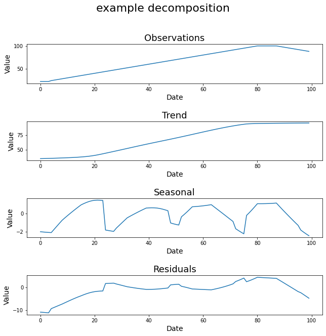
Timeseries Decomposition

STL_decomposition function decomposes the given timeseries into trend, seasonal, and residual components.

The example code:

"""
Created on Thu Apr  1 14:41:53 2021

@author: arsii
"""

import pandas as pd

from tscfat.Analysis.decompose_timeseries import STL_decomposition

# load a dataframe and convert the index to datetime
df = pd.read_csv('/home/arsii/tscfat/Data/Test_data.csv',index_col=0)
df.index = pd.to_datetime(df.index)

# timeseries has to be a numpy array
series = df.level.values

_ = STL_decomposition(series,
                        title = 'example decomposition',
                        test = False,
                        savepath = False,
                        savename = False,
                        ylabel = "Value",
                        xlabel  = "Date",
                        dates = False,
                        )

The output image:

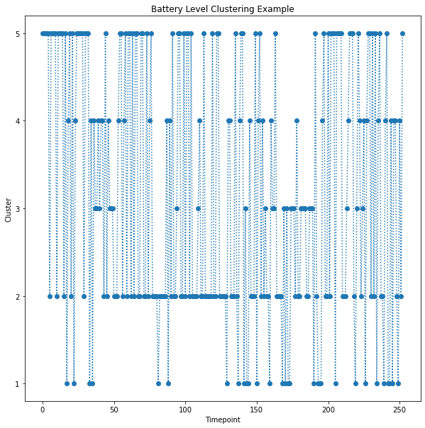
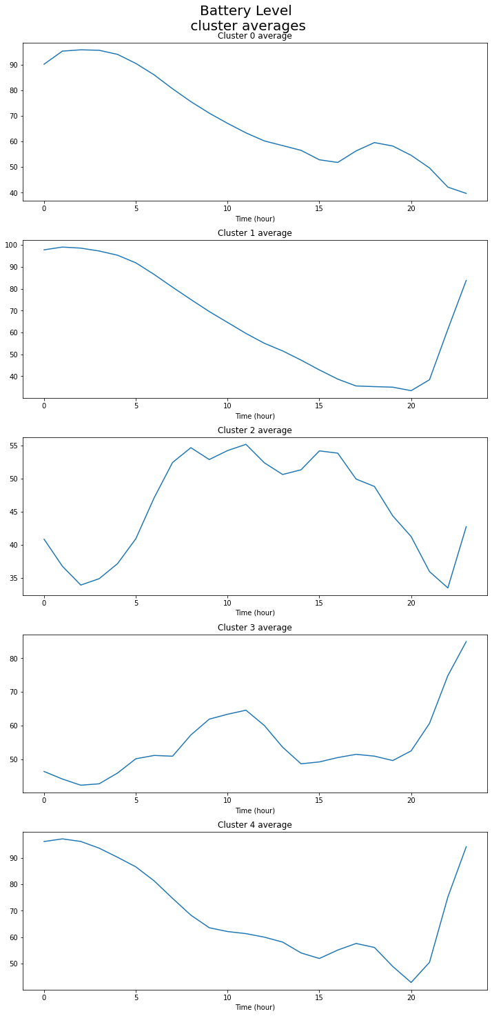
Timeseries Clustering

The example code:

"""
Created on Tue Apr  6 14:01:11 2021

@author: arsii
"""

import pandas as pd
import numpy as np

from tscfat.Analysis.cluster_timeseries import cluster_timeseries

# Load the data and convert index into Datetime
df = pd.read_csv('/home/arsi/Documents/tscfat/Data/Battery_test_data.csv',index_col=0)
df.index = pd.to_datetime(df.index)

df = df.resample('H').mean()

df = df.interpolate()

df = df.resample('D').apply(list)

df = df[1:-1]

data = np.stack(df.battery_level.values)

clusters = cluster_timeseries(data,
                              FIGNAME = False,
                              FIGPATH = False,
                              title = 'Battery Level',
                              n = 5,
                              mi = 5,
                              mib = 5,
                              rs = 0,
                              metric = 'dtw',
                              highlight = None,
                              ylim_ = (0,100)
                              )

The output images:

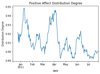
Degree of Distribution

The example code:

"""
Created on Mon Apr  5 21:18:34 2021

@author: arsi
"""

import pandas as pd

from tscfat.Analysis.degree_of_distribution import distribution_degree

# load a dataframe and convert the index to datetime
df = pd.read_csv('/home/arsi/Documents/tscfat/Data/one_subject_data.csv',index_col=0)
df.index = pd.to_datetime(df.index)

# set range of fluctuation
scale = 1

# window
w = 14

# calculate distribution degree
dist_deg = df.positive.rolling(window = w).apply(lambda x: distribution_degree(x.values,scale,w))

# plot the result
ax = dist_deg.plot()
ax.set(ylabel='Distribution Degree', title="Positive Affect Distribution Degree")

The output image:

Fluctuation Intensity

The example code:

"""
Created on Sat Apr  3 23:48:38 2021

@author: arsi
"""

import pandas as pd

from tscfat.Analysis.fluctuation_intensity import fluctuation_intensity

# load a dataframe and convert the index to datetime
df = pd.read_csv('/home/arsi/Documents/tscfat/Data/one_subject_data.csv',index_col=0)
df.index = pd.to_datetime(df.index)

# set range of fluctuation
scale = 1

# window
w = 14

# calculate fluctuation intensity
flu_int = df.positive.rolling(window = w).apply(lambda x: fluctuation_intensity(x.values,scale,w))

# plot the result
ax = flu_int.plot()
ax.set(ylabel='Fluctuation Intensity', title="Positive Affect Fluctuation Intensity")

The output image:

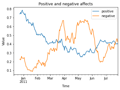
Plot Timeseries

The example code:

"""
Created on Fri Apr  2 12:14:27 2021

@author: arsi
"""

import pandas as pd

from tscfat.Analysis.plot_timeseries import plot_timeseries

# load a dataframe and convert the index to datetime
df = pd.read_csv('/home/arsi/Documents/tscfat/Data/one_subject_data.csv',index_col=0)
df.index = pd.to_datetime(df.index)

# A list containing column names
cols = ['positive','negative']

# Rolling window size
window = 14


_ = plot_timeseries(df,
                    cols,
                    title = 'Positive and negative affects',
                    roll = window,
                    xlab = "Time",
                    ylab = "Value",
                    ylim = False,
                    savename = False,
                    savepath = False,
                    highlight = False,
                    test = False
                    )

The output image:

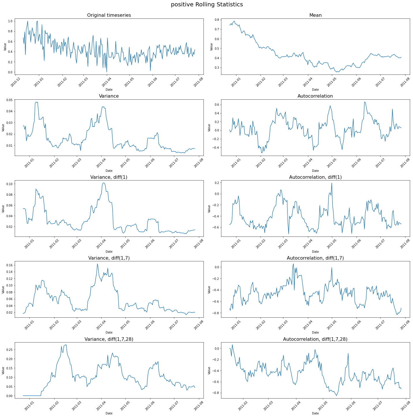
Rolling Statistics

The example code:

import pandas as pd

from tscfat.Analysis.rolling_statistics import rolling_statistics

# load a dataframe and convert the index to datetime
df = pd.read_csv('/home/arsii/tscfat/Data/one_subject_data.csv',index_col=0)
df.index = pd.to_datetime(df.index)

# dataframe can contain only one column
df = df.filter(['positive'])

# rolling window length
window = 14

_ = rolling_statistics(df,
                       window,
                       doi = None,
                       savename = False,
                       savepath = False,
                       test = False,
                       )

The output image:

Summary Statistics

The example code:

"""
Created on Mon Apr  5 21:40:44 2021

@author: arsi
"""

import pandas as pd

from tscfat.Analysis.summary_statistics import summary_statistics

# load a dataframe and convert the index to datetime
df = pd.read_csv('/home/arsi/Documents/tscfat/Data/one_subject_data.csv',index_col=0)
df.index = pd.to_datetime(df.index)

# Select 'Positive' column and convert it into pandas series
ser = df['positive']

# Rolling window size
w = 14

_ = summary_statistics(ser,
                       title = "Time series summary",
                       window = w,
                       savepath = False,
                       savename = False,
                       test = False,
                       )

The output image: